Forecast the future in a timeseries data with Deep Java Library (DJL)
-- Demonstration on M5forecasting and airpassenger datasests
Junyuan Zhang, Kexin Feng
Time series data are commonly seen in the world. They can contain valued information that helps forecast for the future, monitor the status of a procedure and feedforward a control. Generic applications includes the following: sales forecasting, stock market analysis, yield projections, process and quality control, and many many more. See link1 and link2 for further examples of timeseries data.
The timeseries package introduced here belongs to a deep learning framework, DeepJavaLibrary DJL. It is designed for Java developers and is compatible with the existing popular deep learning engines, like PyTorch, MXNet, and Tensorflow. This library enables users to easily train and deploy deep learning models in their Java application. The package contains the following two major features.
- It integrates DJL with gluonTS, a powerful timeseries python package. With this feature, the pretrained models in gluonTS, either with MXNet or PyTorch, can both be directly loaded into DJL for inference and deployment in Java environment. Also take a look at the python example m5_gluonts_template. Our convention of the parameter names are the same as theirs.
- It contains training features, so that users can directly build and modify timeseries deep learning models in DJL within Java envinronment.
In the following, we will demonstrate these features with M5 Forecasting data. We will also use the airpassenger data to benchmark the pretrained model loaded from gluonTS. The example is structured as follows.
- A simple demonstration with airpassenger data
- M5 Forecasting dataset
- DeepAR model
- Inference feature: inference with pretrained DeepAR model.
- Training feature: build and train your own DeepAR model
- Summary
A simple demonstration with airpassenger data
We start with a simple demonstration of the DeepAR model applied on the airpassenger data, to get a sense of its performance. The dataset consists of a single time series, containing monthly international passengers between the years 1949 and 1960, a total of 144 values (12 years * 12 months). The model is pretrained in gluonTS and then directly loaded into DJL. The source code is here.
The result is shown in the graph below. It has the same performance as shown in gluonTS website. We can see the historical pattern is effectively learned as manifested in its forecast. Next, you will see how to easily apply this model on a more realistic data in M5 forecasting task.

M5 Forecasting dataset
This demonstration is based on the Kaggle M5 Forecasting competition. The dataset contains 42,840 hierarchical time-series data of the unit sales of Walmart retail goods. “Hierarchical” here means that we can aggregate the data from different perspectives, including item level, department level, product category level, and state level. Also for each item, we can access information about its price, promotions, and holidays. As well as sales data from Jan 2011 all the way to June 2016.
Note. In the original M5 forecasting data, the time series data is very sparse containing many zero values. These zero can be seen as inactive data. So
we aggregate the sales by week to train and predict at a coarser granularity, which focues on only the active data. To also predict for the inactive data, another model may be needed to be combined. The data aggration is done with a python script m5_data_coarse_grain.py. This script will create weekly_xxx.csv files representing weekly data in the dataset directory you specify.
DeepAR model
DeepAR forecasting algorithm is a supervised learning algorithm for forecasting scalar (one-dimensional) time series using recurrent neural networks (RNN). Unlike traditional time series forecasting models, DeepAR estimates the future probability distribution instead of a specific number. In retail businesses, probabilistic demand forecasting is critical to delivering the right inventory at the right time and in the right place. Therefore, we choose the sales data set in the real scene as an example to describe how to use the timeseries package for forecasting.
Also take a look at the python example m5_gluonts_template for the demonstration of DeepAR model. Our convention of the parameter names are the same as theirs.
Inference feature: inference with pretrained DeepAR model
Setup
To get started with DJL time series package, add the following code snippet defining the necessary dependencies to your build.gradle file.
plugins {
  id 'java'
}
repositories {
  mavenCentral()
}
dependencies {
  implementation "org.apache.logging.log4j:log4j-slf4j-impl:2.17.1"
  implementation platform("ai.djl:bom:0.27.0")
  implementation "ai.djl:api"
  implementation "ai.djl.timeseries"
  runtimeOnly "ai.djl.mxnet:mxnet-engine"
  runtimeOnly "ai.djl.mxnet:mxnet-model-zoo"
}
Define your dataset
In order to realize the preprocessing of time series data, we define the TimeSeriesData as the input of the Translator, which is used to store the feature fields and perform corresponding transformations.
So for your own dataset, you need to customize the way you get the data and put it into TimeSeriesData as the input to the translator. In this demo, we use M5Dataset which is located in M5ForecastingDeepAR.java.
The dataset path is set in the follwing code.
Repository repository = Repository.newInstance("local_dataset",
    Paths.get("YOUR_PATH/m5-forecasting-accuracy"));
NDManager manager = NDManager.newBaseManager();
M5Dataset dataset = M5Dataset.builder().setManager(manager).optRepository(repository).build();
Configure your translator and load the local model
The inference workflow consists of input pre-processing, model forward, and output post-processing. DJL encapsulates input and output processing into the translator, and uses Predictor to do the model forward.
DeepARTranslator provides support for data preprocessing and postprocessing for probabilistic prediction models. Similar to GluonTS, this translator is specifically designed for the timeseriesData, which fetches the data according to different parameters, like frequency, which are configured as shown below. For any other GluonTS model, you can quickly develop your own translator using the classes in transform modules (etc. TransformerTranslator).
Here, the Criteria API is used as search criteria to look for a ZooModel. In this application, you can customize your local pretrained model path: /YOUR PATH/deepar.zip .
String modelUrl = "YOUR_PATH/deepar.zip";
int predictionLength = 4;
Criteria<TimeSeriesData, Forecast> criteria =
        Criteria.builder()
                .setTypes(TimeSeriesData.class, Forecast.class)
                .optModelUrls(modelUrl)
                .optEngine("MXNet") // or PyTorch
                .optTranslatorFactory(new DeferredTranslatorFactory())
                .optArgument("prediction_length", predictionLength)
                .optArgument("freq", "W")
                .optArgument("use_feat_dynamic_real", "false")
                .optArgument("use_feat_static_cat", "false")
                .optArgument("use_feat_static_real", "false")
                .optProgress(new ProgressBar())
                .build();
Note: Here the arguments predictionLength and freq decide the structure of the model. So for a specific model, these two arguments cannot be changed, such that the translator is compatible with the models in terms of the tensor shapes.
Also note that, for a model exported from MXNet, the tensor shape of the begin_state may be problematic, as indicated in this issue. As described there, you need to "change every begin_state's shape to (-1, 40)". Otherwise the model would not allow batch data processing.
Prediction
Now, you are ready to use the model bundled with the translator created above to run inference.
Since we need to generate features based on dates and make predictions with reference to the context, for each TimeSeriesData you must set the values of its StartTime and TARGET fields.
try (ZooModel<TimeSeriesData, Forecast> model = criteria.loadModel();
             Predictor<TimeSeriesData, Forecast> predictor = model.newPredictor()) {
    data = dataset.next();
    NDArray array = data.singletonOrThrow();
    TimeSeriesData input = new TimeSeriesData(10);
    input.setStartTime(startTime);  // start time of prediction
    input.setField(FieldName.TARGET, array);  // target value through whole context length
    Forecast forecast = predictor.predict(input);

    // save data for plotting
    NDArray target = input.get(FieldName.TARGET);
    target.setName("target");
    saveNDArray(target);

    // Save data for plotting.
    NDArray samples = ((SampleForecast) forecast).getSortedSamples();
    samples.setName("samples");
    saveNDArray(samples);
}
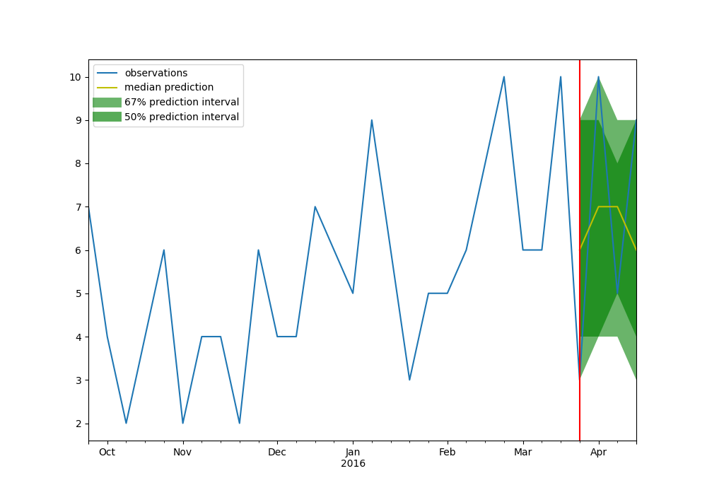
Results
The Forecast are objects that contain all the sample paths in the form of NDArray with dimension (numSamples, predictionLength), the start date of the forecast. You can access all these information by simply invoking the corresponding function.
You can summarize the sample paths by computing, including the mean and quantile, for each step in the prediction window.
logger.info("Mean of the prediction windows:\n" + forecast.mean().toDebugString());
logger.info("0.5-quantile(Median) of the prediction windows:\n" + forecast.quantile("0.5").toDebugString());
> [INFO ] - Mean of the prediction windows:
> ND: (4) cpu() float32
> [5.97, 6.1 , 5.9 , 6.11]
>
> [INFO ] - 0.5-quantile(Median) of the prediction windows:
> ND: (4) cpu() float32
> [6., 5., 5., 6.]
We visualize the forecast result with mean, prediction intervals, etc. The plot function is in a python script plot.py.
Metrics
We use the following metrics to evaluate the performance of the DeepAR model in the M5 Forecasting competition.
> [INFO ] - metric: Coverage[0.99]:    0.92
> [INFO ] - metric: Coverage[0.67]:    0.51
> [INFO ] - metric: abs_target_sum:    1224665.00
> [INFO ] - metric: abs_target_mean:   10.04
> [INFO ] - metric: NRMSE: 0.84
> [INFO ] - metric: RMSE:  8.40
> [INFO ] - metric: RMSSE: 1.00
> [INFO ] - metric: abs_error: 14.47
> [INFO ] - metric: QuantileLoss[0.67]:    18.23
> [INFO ] - metric: QuantileLoss[0.99]:    103.07
> [INFO ] - metric: QuantileLoss[0.50]:    9.49
> [INFO ] - metric: QuantileLoss[0.95]:    66.69
> [INFO ] - metric: Coverage[0.95]:    0.87
> [INFO ] - metric: Coverage[0.50]:    0.33
> [INFO ] - metric: MSE:   70.64
Here, we focus on the metric Root Mean Squared Scaled Error, ie. RMSSE. The detailed formula is in here. It is different from the Root-mean-square error RMSE in that RMSSE is based on the variation between two contiguous data points. So this metric is scale invariant, suitable for timeseries data.
As you can see, in the result metric above, the model has RMSSE = 1.00. This means that, on average, the error
between the prediction and the actual data is around 1.00 time the average variation of the timeseries. This is also
seen in the
result graph above: the predicted intervals are about the same as the data variation over time. If the predicted interval were smaller, then the prediction would be more accurate, like the plot with the airpassenger data in the second next section. In the Kaggle contest learderboard, the best model can reach RSSSM = 0.5.
Click here to see the source code of the inference feature.
Training feature: build and train your own DeepAR model
In this section we will take you through the creation and training of our time series model — DeepAR.
Define your probability distribution
In timeseries package, we do not just predict the target value, but the target probability distribution. The parameter of the probablity distribution will be contained in the loss function. So this can be seen as parametric statistics.
The benifit of using probability distribution is that it can reflect the possibility of the target value in different intervals, which is of greater significance for real production scenarios. Therefore, before you train any of your timing models, you need to define a probability DistributionOutput for it as the predicted output.
DistributionOutput distributionOutput = new NegativeBinomialOutput();
Here we consider that sales are more in line with the negtive binomial distribution.
Construct your model
As with Translator you need to set some hyperparameters, including the frequency, length of the prediction even number of layers for a neural network, etc.
String freq = "W";
int predictionLength = 4;
DeepARNetwork getDeepARModel(DistributionOutput distributionOutput, boolean training) {
    DeepARNetwork.Builder builder = DeepARNetwork.builder()
        .setCardinality(cardinality)
        .setFreq(freq)
        .setPredictionLength(predictionLength)
        .optDistrOutput(distributionOutput)
        .optUseFeatStaticCat(true);
    // This is because the network will output different content during training and inference
    return training ? builder.buildTrainingNetwork() : builder.buildPredictionNetwork();
After we set up the configuration, we can build a DeepAR Network Block and set it back to model using setBlock
Model model = Model.newInstance("deepar");
DeepARNetwork trainingNetwork = getDeepARModel(distributionOutput, true);
model.setBlock(trainingNetwork);
Prepare dataset
For TimeseriesDataset, you need to specify the pre-processing transformations, which includes steps such as time-series feature generation and transformation that need to be applied to TimeSeriesData before feeding the input to the model.
Different models have different pre-processing requirements, so we can derive the corresponding transformations based on the previously obtained network models and obtain some necessary parameters.
List<TimeSeriesTransform> trainingTransformation = trainingNetwork.createTrainingTransformation(manager);
int contextLength = trainingNetwork.getContextLength();
You can construct a M5Forecast builder with your own specifications.
M5Forecast getDataset(
    List<TimeSeriesTransform> transformation,
    Repository repository,
    int contextLength,
    Dataset.Usage usage) {
    // In order to create a TimeSeriesDataset, you must specify the transformation of the data
    // preprocessing
    M5Forecast.Builder builder =
        M5Forecast.builder()
        .optUsage(usage)
        .setRepository(repository)
        .setTransformation(transformation)
        .setContextLength(contextLength)
        .setSampling(32, usage == Dataset.Usage.TRAIN);

    int maxWeek = usage == Dataset.Usage.TRAIN ? 273 : 277;
    for (int i = 1; i <= maxWeek; i++) {
        builder.addFeature("w_" + i, FieldName.TARGET);
    }

    // This is the static category feature
    M5Forecast m5Forecast =
        builder.addFeature("state_id", FieldName.FEAT_STATIC_CAT)
        .addFeature("store_id", FieldName.FEAT_STATIC_CAT)
        .addFeature("cat_id", FieldName.FEAT_STATIC_CAT)
        .addFeature("dept_id", FieldName.FEAT_STATIC_CAT)
        .addFeature("item_id", FieldName.FEAT_STATIC_CAT)
        .addFieldFeature(
        FieldName.START,
        // A Featurizer convert String to LocalDateTime
        new Feature("date", TimeFeaturizers.getConstantTimeFeaturizer(startTime)))
        .build();
    m5Forecast.prepare(new ProgressBar());
    return m5Forecast;
}
Set up training configuration
We need to set the loss function of the model in this section, and for any probability distribution, the corresponding loss needs to be calculated by DistributionLoss wrapping.
DefaultTrainingConfig setupTrainingConfig(
            Arguments arguments, DistributionOutput distributionOutput) {
    return new DefaultTrainingConfig(new DistributionLoss("Loss", distributionOutput))
        .addEvaluator(new RMSSE(distributionOutput)) // Use RMSSE so we can understand the performance of the model
        .optDevices(Engine.getInstance().getDevices(arguments.getMaxGpus()))
        .optInitializer(new XavierInitializer(), Parameter.Type.WEIGHT);
}
Model training
Now you can start training.
Repository repository = Repository.newInstance("test",Paths.get("YOUR PATH"));
M5Forecast trainSet = getDataset(trainingTransformation, repository, contextLength, Dataset.Usage.TRAIN);

Trainer trainer = model.newTrainer(config)
trainer.setMetrics(new Metrics());

int historyLength = trainingNetwork.getHistoryLength();
Shape[] inputShapes = new Shape[9];
// (N, num_cardinality)
inputShapes[0] = new Shape(1, 5);
// (N, num_real) if use_feat_stat_real else (N, 1)
inputShapes[1] = new Shape(1, 1);
// (N, history_length, num_time_feat + num_age_feat)
inputShapes[2] =new Shape(1, historyLength, TimeFeature.timeFeaturesFromFreqStr(freq).size() + 1);
inputShapes[3] = new Shape(1, historyLength);
inputShapes[4] = new Shape(1, historyLength);
inputShapes[5] = new Shape(1, historyLength);
inputShapes[6] = new Shape(1,predictionLength, TimeFeature.timeFeaturesFromFreqStr(freq).size() + 1);
inputShapes[7] = new Shape(1, predictionLength);
inputShapes[8] = new Shape(1, predictionLength);
trainer.initialize(inputShapes);

int epoch = 10;
EasyTrain.fit(trainer, epoch, trainSet, null);
After you have completed the above process, you will see the following information:
[INFO ] - Training on: cpu().
[INFO ] - Load MXNet Engine Version 1.9.0 in 0.086 ms.
Training:     30% |=============                           | RMSSE: 1.43, Loss: 2.42, speed: 443.11 items/sec
The java source code of this training example is TrainTimeSeries.java. For your reference, the counterpart python source code for training is also available in 5torch.py
Summary
In this example, we have shown the DJL timeseries package with M5 Forecasting data. We focuse on the inference feature, but the training feature is also available here, where you can build your own timeseries model in DJL. With these features in DJL, now users can start mining the timeseriese data conveniently in Java.