Train ResNet for Fruit Freshness Classficiation
Deep learning has shown its strong power in solving problems in various areas like CV, NLP, reinforcement learning, etc., which generates numerous examples of successful applications. However, for a very specific customized task, like rotten fruit detection in a grocery store, or mask wearing detection in a public place, there are still many challenges to face, including the following two: 1. The training dataset suitable for the task is usually not immediately available, while data collection and annotation can be expensive. 2. Training a model from scratch can be time-consuming and may face many uncertainties.
In this example, we will address the above two issues with transfer learning, and demonstrate it on a rotten fruit detection task. Our result shows that the model can achieve 95% accuracy on image classification with less than 100 images. We will also show how easily this is implemented in Java environment. You will learn how this is achieved in the next 10 minutes.
To solve the issues mentioned above, we will use the transfer learning feature in DJL. We will also use ATLearn, an adaptive transfer learning toolkit, to edit and import the large pre-train model. ATLearn is a light weighted transfer learning toolkit, with various APIs, algorithms and model zoo, provided for python users.
The example is structured as follows: 1. The data set and the problem formulation 2. The transfer learning model 3. The demonstration of transfer learning in Java 4. Experiment on the reduction of the training data size
The full source code is available here.
The data set and the problem formulation
In this example, we demonstrate with the fruit fresh and rotten dataset, which is publicly available from Kaggle contest. This dataset is composed of pictures with one fruit in it, either fresh or rotten. So, the task of detecting the rotten fruit can be formulated as a 2-class classification problem. This task has a potential application in grocery store in building automatic rotten fruit detection.
Here are some examples of the image data.
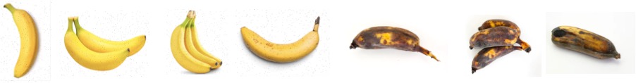
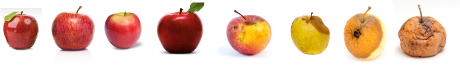
It is then clear that the fruit images indeed have enough visual variation distinguishable for a classifier model.
The transfer learning model
Based on transfer learning, the model is built on top of a large pre-trained model, which is used to get an embedding vector. Then the embedding vector is fed into the subsequent fully connected layer followed by a SoftMax activation function. Thus, through transfer learning, users can benefit from the large pre-trained model and solve their own customized problem.
The pretrained model used in this demonstration is ResNet18. You can obtain an embedding model made of it from ATLearn, or manually from PyTorch. Here we show the method using ATLearn, where the embedding model can be directly exported.
import ATLearn
model = ATLearn.get_embedding(ATLearn.task.IMAGE_CLASSIFICATION,
                              "EXPORT_PATH",
                              network='resnet18',  # pre-trained model from torch
                              user_network=None)   # users' own pre-trained model
At this step, what ATLearn does is to remove the last layer of ResNet18 to get the intermediate
vector, and then to trace and export the model as a TorchScript file resnet18_embedding.pt,
which can then be directly loaded in DJL. This part will be introduced in the next section.
The demonstration of transfer learning in Java
Overall, this transfer learning feature is a training feature, so its API shares similarities to other DJL training examples. It mainly contains model structure, data loading, training configuration and metric.
Model building
Load the embedding in DJL and build the model. As mentioned before, we have generated an
embedding layer from ATLearn. Now we can load it into DJL. This embedding layer is also available
at modelUrl = "djl://ai.djl.pytorch/resnet18_embedding". In DJL, the model loading is implemented
with the criteria API, which serves as the criteria to search for models. It offers several
options to configure the model. Among them, trainParam is an option specific for transfer
learning (or model retraining). Setting it "false" will freeze the parameter in the loaded
embedding layer (or model), and "true" will be the other way around.
String modelUrl = "/EXPORT_PATH/resnet18_embedding.pt";
Criteria<NDList, NDList> criteria = Criteria.builder()
        .setTypes(NDList.class, NDList.class)
        .optModelUrls(modelUrl)
        .optEngine("PyTorch")
        .optProgress(new ProgressBar())
        .optOption("trainParam", "true")  // or "false" to freeze the embedding
        .build();
ZooModel<NDList, NDList> embedding = criteria.loadModel();
Block baseBlock = embedding.getBlock();
On top of the embedding model, we further add a fully connected (FC) layer (also denoted as MLP layer), the output dimension of which is the number of classes, i.e., 2 in this task. We use a sequential block model to contain the embedding and fully connected layer. The final output is a SoftMax function to get class probability, as shown below.
Block blocks = new SequentialBlock()
        .add(baseBlock)
        .addSingleton(nd -> nd.squeeze(new int[] {2, 3}))  // squeeze the size-1 dimensions from the baseBlock
        .add(Linear.builder().setUnits(2).build()) // add fully connected layer
        .addSingleton(nd -> nd.softmax(1));
Model model = Model.newInstance("TransferFreshFruit");
model.setBlock(blocks);
Trainer configuration. The configuration of trainer mainly contains the settings of loss
function (SoftmaxCrossEntropy in this case), the evaluation metric (Accuracy in this case),
training listener which is used to fetch the training monitoring data, and so on. In our task,
they are specified as shown below.
private static DefaultTrainingConfig setupTrainingConfig(Block baseBlock) {
    String outputDir = "build/fruits";
    SaveModelTrainingListener listener = new SaveModelTrainingListener(outputDir);
    listener.setSaveModelCallback(
            trainer -> {
                TrainingResult result = trainer.getTrainingResult();
                Model model = trainer.getModel();
                float accuracy = result.getValidateEvaluation("Accuracy");
                model.setProperty("Accuracy", String.format("%.5f", accuracy));
                model.setProperty("Loss", String.format("%.5f", result.getValidateLoss()));
            });

    DefaultTrainingConfig config = new DefaultTrainingConfig(new SoftmaxCrossEntropy("SoftmaxCrossEntropy"))
            .addEvaluator(new Accuracy())
            .optDevices(Engine.getEngine("PyTorch").getDevices(1))
            .addTrainingListeners(TrainingListener.Defaults.logging(outputDir))
            .addTrainingListeners(listener);
     ...
     return config;
}
At this step, we will assign different learning rates on these two layers: the learning rate of
the embedding layer is 10 times smaller than that of the FC layer. Thus, the pretrained parameters
in the embedding layer is not changed too much. This assignment of learning rate is specified with
learningRateTracker, which is then fed into the learningRateTracker option in Optimizer,
as shown below.
// Customized learning rate
float lr = 0.001f;
FixedPerVarTracker.Builder learningRateTrackerBuilder = FixedPerVarTracker.builder().setDefaultValue(lr);
for (Pair<String, Parameter> paramPair : baseBlock.getParameters()) {
    learningRateTrackerBuilder.put(paramPair.getValue().getId(), 0.1f * lr);
}
FixedPerVarTracker learningRateTracker = learningRateTrackerBuilder.build();
Optimizer optimizer = Adam.builder().optLearningRateTracker(learningRateTracker).build();
config.optOptimizer(optimizer);
After this step, a training configuration is returned by setupTrainingConfig function. It is then
used to set the trainer.
Trainer trainer = model.newTrainer(config);
Next, the trainer is initialized by the following code, where the parameters' shape and initial
value in each block will be specified. The inputShape has to be known beforehand.
int batchSize = 32;
Shape inputShape = new Shape(batchSize, 3, 224, 224);
trainer.initialize(inputShape);
Data loading. The data is loaded and preprocessed with the following function.
private static RandomAccessDataset getData(String usage, int batchSize)
        throws TranslateException, IOException {
    float[] mean = {0.485f, 0.456f, 0.406f};
    float[] std = {0.229f, 0.224f, 0.225f};

    // usage is either "train" or "test"
    Repository repository = Repository.newInstance("banana", Paths.get("LOCAL_PATH/banana/" + usage));
    FruitsFreshAndRotten dataset = FruitsFreshAndRotten.builder()
            .optRepository(repository)
            .addTransform(new RandomResizedCrop(256, 256)) // only in training
            .addTransform(new RandomFlipTopBottom()) // only in training
            .addTransform(new RandomFlipLeftRight()) // only in training
            .addTransform(new Resize(256, 256))
            .addTransform(new CenterCrop(224, 224))
            .addTransform(new ToTensor())
            .addTransform(new Normalize(mean, std))
            .addTargetTransform(new OneHot(2))
            .setSampling(batchSize, true)
            .build();
    dataset.prepare();
    return dataset;
}
Here, the data are preprocessed with the normalization and randomization functions, which are commonly used for image classification. The randomization are for training only.
Model training and export. Finally, we can run the model training with Easytrain.fit,
and save the model for prediction. In the end, the model.close() and embedding.close()
are called. In DJL, during the creation of Model and ZooModel<NDList, NDList>, the native
resources (e.g., memories in the assigned in PyTorch) are allocated. These resources are managed
by NDManager which inherits AutoCloseable class.
EasyTrain.fit(trainer, numEpoch, datasetTrain, datasetTest);
model.save(Paths.get("SAVE_PATH"), "transferFreshFruit");

model.close();
embedding.close();
When running the training code, the VM option needs to be set -Dai.djl.default_engine=PyTorch
to specify the engine. The generic output of the training process will be the following:
Training:    100% |████████████████████████████████████████| speed: 28.26 items/sec
Validating:  100% |████████████████████████████████████████|
[INFO ] - Epoch 10 finished.
[INFO ] - Train: Accuracy: 0.93, SoftmaxCrossEntropy: 0.22
[INFO ] - Validate: Accuracy: 0.90, SoftmaxCrossEntropy: 0.34
Here, you can monitor the training and validation accuracy and loss descent.
Experiment on the reduction of the training data size
The key advantage of transfer learning is that it leverages the pretrained model, and thus it can
be trained on a relatively small dataset. This will save the cost in data collection and
annotation. In this section, we measure the validation accuracy vs. training data size on
the FreshFruit dataset. The full experiment code is available
here.
In this experiment, the training dataset size needs to be controlled and randomly chosen.
This part is implemented as below, where cut is the size of the training data.
List<Long> batchIndexList = new ArrayList<>();
try (NDManager manager = NDManager.newBaseManager()) {
    NDArray indices = manager.randomPermutation(dataset.size());
    NDArray batchIndex = indices.get(":{}", cut);
    for (long index : batchIndex.toLongArray()) {
        batchIndexList.add(index);
    }
}
return dataset.subDataset(batchIndexList);
The result of validation accuracy v.s. training data size is below.
![]()
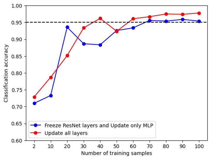
Here, we have tested two scenarios: freeze ResNet layers and update only MLP and update all layers. As expected, the stable accuracy of latter is slightly better than that of the former, since the ResNet parameter is also fine-tuned by the data. We can also see that the accuracy of the banana data reaches stable 0.95 with 30 samples, the accuracy of the apple data reaches stable 0.95 with around 70 samples. They are both relatively smaller than the provided training data size by Kaggle, which is over 1000. This verifies that, indeed the required training dataset is small. When people need to collect and annotate data, this offers a reference on the minimum required data size.
Summary
In this example, we demonstrate how to build a transfer learning model in DJL for an image classification task. This process is also applicable in model retraining. Finally, we also present the experiment on how much the training data set can be reduced. The direct benefit of the reduced is that it helps to save the expensive data collection and annotation cost. This makes it much easier to leverage the large pretrained models to solve other various tasks with small dataset.
This demonstration is similarly applied to other tasks and data, like mask wearing detection and fruit freshness regression. See examples in ATLearn for their implementation in python, as well as other examples of object detection.